Lebesgue integration
2008/9 Schools Wikipedia Selection. Related subjects: Mathematics

In mathematics, the integral of a nonnegative function can be regarded in the simplest case as the area between the graph of that function and the x-axis. Lebesgue integration is a mathematical construction that extends the integral to a larger class of functions; it also extends the domains on which these functions can be defined. It had long been understood that for nonnegative functions with a smooth enough graph (such as continuous functions on closed bounded intervals) the area under the curve could be defined as the integral and computed using techniques of approximation of the region by polygons. However, as the need to consider more irregular functions arose (for example, as a result of the limiting processes of mathematical analysis and the mathematical theory of probability) it became clear that more careful approximation techniques would be needed in order to define a suitable integral.
The Lebesgue integral plays an important role in the branch of mathematics called real analysis and in many other fields in the mathematical sciences.
The Lebesgue integral is named for Henri Lebesgue (1875-1941). His last name is pronounced [ləˈbɛg], approximately luh beg.
The term "Lebesgue integration" may refer either to the general theory of integration of a function with respect to a general measure, as introduced by Lebesgue, or to the specific case of integration of a function defined on a sub-domain of the real line with respect to Lebesgue measure.
Introduction
The integral of a function f between limits a and b can be interpreted as the area under the graph of f. This is easy to understand for familiar functions such as polynomials, but what does it mean for more exotic functions? In general, what is the class of functions for which "area under the curve" makes sense? The answer to this question has great theoretical and practical importance.
As part of a general movement toward rigour in mathematics in the nineteenth century, attempts were made to put the integral calculus on a firm foundation. The Riemann integral, proposed by Bernhard Riemann (1826-1866), is a broadly successful attempt to provide such a foundation for the integral. Riemann's definition starts with the construction of a sequence of easily-calculated integrals which converge to the integral of a given function. This definition is successful in the sense that it gives the expected answer for many already-solved problems, and gives useful results for many other problems.
However, Riemann integration does not interact well with taking limits of sequences of functions, making such limiting processes difficult to analyze. This is of prime importance, for instance, in the study of Fourier series, Fourier transforms and other topics. The Lebesgue integral is better able to describe how and when it is possible to take limits under the integral sign. The Lebesgue definition considers a different class of easily-calculated integrals than the Riemann definition, which is the main reason the Lebesgue integral is better behaved. The Lebesgue definition also makes it possible to calculate integrals for a broader class of functions. For example, the Dirichlet function, which is 0 where its argument is irrational and 1 otherwise, has a Lebesgue integral, but it does not have a Riemann integral.
Construction of the Lebesgue integral
The discussion that follows parallels the most common expository approach to the Lebesgue integral. In this approach the theory of integration has two distinct parts:
- A theory of measurable sets and measures on these sets.
- A theory of measurable functions and integrals on these functions.
Measure theory
Measure theory initially was created to provide a detailed analysis of the notion of length of subsets of the real line and more generally area and volume of subsets of Euclidean spaces. In particular, it provided a systematic answer to the question of which subsets of R have a length. As was shown by later developments in set theory (see non-measurable set), it is actually impossible to assign a length to all subsets of R in a way which preserves some natural additivity and translation invariance properties. This suggests that picking out a suitable class of measurable subsets is an essential prerequisite.
Of course, the Riemann integral uses the notion of length implicitly. Indeed, the element of calculation for the Riemann integral is the rectangle [a, b] × [c, d], whose area is calculated to be (b−a)(d−c). The quantity b−a is the length of the base of the rectangle and d−c is the height of the rectangle. Riemann could only use planar rectangles to approximate the area under the curve because there was no adequate theory for measuring more general sets.
In the development of the theory in most modern textbooks (after 1950), the approach to measure and integration is axiomatic. This means that a measure is any function μ defined on certain subsets X of a set E which satisfies a certain list of properties. These properties can be shown to hold in many different cases.
The theory of measurable sets and measure (including definition and construction of such measures) is discussed in other articles. See measure.
Integration
As usual we start with a measure space, (E,X,μ). In this, E is just a set, X is a σ-algebra of subsets of E and μ is a (non-negative) measure on X of subsets of E.
For example, E can be Euclidean n-space Rn or some Lebesgue measurable subset of it, X will be the σ-algebra of all Lebesgue measurable subsets of E, and μ will be the Lebesgue measure. In the mathematical theory of probability μ will be a probability measure on a probability space E.
In Lebesgue's theory, integrals are limited to a class of functions called measurable functions. A function f is measurable if the pre-image of every closed interval is in X:
![f^{-1}([a,b]) \in X \mbox{ for all }a<b.](../../images/174/17492.png)
It can be shown that this is equivalent to requiring that the pre-image of any Borel subset of R be in X. We will make this assumption from now on. The set of measurable functions is closed under algebraic operations, but more importantly the class is closed under various kinds of pointwise sequential limits:
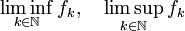
are measurable if the original sequence {fk}, where k  N, consists of measurable functions.
We build up an integral

for measurable real-valued functions f defined on E in stages:
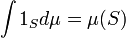
Indicator functions: To assign a value to the integral of the indicator function of a measurable set S consistent with the given measure μ, the only reasonable choice is to set:
Simple functions: We extend by linearity to the linear span of indicator functions:
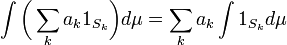
where the sum is finite and the coefficients ak are real numbers. Such a finite linear combination of indicator functions is called a simple function. Even if a simple function can be written in many ways as a linear combination of indicator functions, the integral will always be the same.
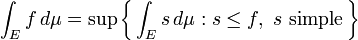
Non-negative functions: Let f be a non-negative measurable function on E which we allow to attain the value +∞, in other words, f takes non-negative values in the extended real number line. We define
We need to show this integral coincides with the preceding one, defined on the set of simple functions. There is also the question of whether this corresponds in any way to a Riemann notion of integration. It is not hard to prove that the answer to both questions is yes.
We have defined the integral of f for any non-negative extended real-valued measurable function on E. For some functions ∫f will be infinite.
Signed functions: To handle signed functions, we need a few more definitions. If f is a function of the measurable set E to the reals (including ± ∞), then we can write
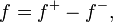
where
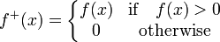
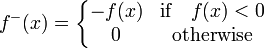
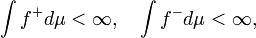
Note that both f+ and f− are non-negative functions. Also note that
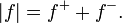
If
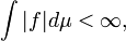
then f is called Lebesgue integrable. In this case, both integrals satisfy
and it makes sense to define
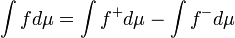
It turns out that this definition gives the desirable properties of the integral.
Complex valued functions can be similarly integrated, by considering the real part and the imaginary part separately.
Intuitive interpretation

To get some intuition about the different approaches to integration, let us imagine that it is desired to find a mountain's volume (above sea level).
The Riemann-Darboux approach: Divide the base of the mountain into a grid of 1 meter squares (a cadaster, in the language of land surveyors). Measure the altitude of the mountain at the centre of each square. The volume on a single grid square is approximately 1x1x(altitude), so the total volume is the sum of the altitudes.
The Lebesgue approach: Draw a contour map of the mountain, where each contour is 1 meter of altitude apart. The volume of earth contained in a single contour is approximately that contour's area times its thickness. So the total volume is the sum of the areas of the contours.
Folland summarizes the difference between the Riemann and Lebesgue approaches thus: "to compute the Riemann integral of f, one partitions the domain [a, b] into subintervals", while in the Lebesgue integral, "one is in effect partitioning the range of f".
Example
Consider the indicator function of the rational numbers, 1Q. This function is nowhere continuous.
 is not Riemann-integrable on [0,1]: No matter how the set [0,1] is partitioned into subintervals, each partition will contain at least one rational and at least one irrational number, since rationals and irrationals are both dense in the reals. Thus the upper Darboux sums will all be one, and the lower Darboux sums will all be zero.
- is Lebesgue-integrable on [0,1] using the Lebesgue measure: Indeed it is the indicator function of the rationals so by definition
![\int_{[0,1]} 1_{\mathbb{Q}} \, d \mu = \mu(\mathbb{Q} \cap [0,1]) = 0,](../../images/175/17509.png)
- since
 is countable.
Limitations of the Riemann integral
Here we discuss the limitations of the Riemann integral and the greater scope offered by the Lebesgue integral. We presume a working understanding of the Riemann integral.
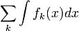
With the advent of Fourier series, many analytical problems involving integrals came up whose satisfactory solution required exchanging infinite summations of functions and integral signs. However, the conditions under which the integrals
 and
and ![\int \bigg[\sum_k f_k(x) \bigg] dx](../../images/175/17512.png)
are equal proved quite elusive in the Riemann framework. There are some other technical difficulties with the Riemann integral. These are linked with the limit taking difficulty discussed above.
Failure of monotone convergence. As shown above, the indicator function 1Q on the rationals is not Riemann integrable. In particular, the Monotone convergence theorem fails. To see why, let {ak} be an enumeration of all the rational numbers in [0,1] (they are countable so this can be done.) Then let
Then let

The function fk is zero everywhere except on a finite set of points, hence its Riemann integral is zero. The sequence fk is also clearly non-negative and monotonically increasing to 1Q, which is not Riemann integrable.
Unsuitability for unbounded intervals. The Riemann integral can only integrate functions on a bounded interval. The simplest extension is to define
whenever the limit exists. However, this breaks the desirable property of translation invariance: if f and g are zero outside some interval [a, b] and are Riemann integrable, and if f(x) = g(x + y) for some y, then ∫ f = ∫ g. With this definition of the improper integral (this definition is sometimes called the improper Cauchy principal value about zero), the functions f(x) = (1 if x > 0, −1 otherwise) and g(x) = (1 if x > 1, −1 otherwise) are translations of one another, but their improper integrals are different.
Basic theorems of the Lebesgue integral
The Lebesgue integral does not distinguish between functions which only differ on a set of μ-measure zero. To make this precise, functions f, g are said to be equal almost everywhere (or equal a.e.) if and only if

- If f, g are non-negative functions (possibly assuming the value +∞) such that f = g almost everywhere, then
- If f, g are functions such that f = g almost everywhere, then f is Lebesgue integrable if and only if g is Lebesgue integrable and the integrals of f and g are the same.
The Lebesgue integral has the following properties:
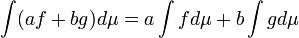
Linearity: If f and g are Lebesgue integrable functions and a and b are real numbers, then af + bg is Lebesgue integrable and
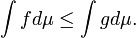
Monotonicity: If f ≤ g, then
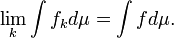
Monotone convergence theorem: Suppose {fk}k ∈ N is a sequence of real, non-negative measurable functions such that

Then
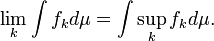
Note: The value of any of the integrals is allowed to be infinite.
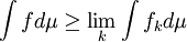
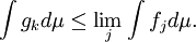
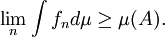
Fatou's lemma: If {fk}k ∈ N is a sequence of real, non-negative measurable functions, then
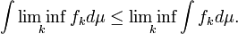
Again, the value of any of the integrals may be infinite.
Dominated convergence theorem: If {fk}k ∈ N is a sequence of complex measurable functions with pointwise limit f, and if there is a Lebesgue integrable function g (i.e, g ∈ L1) such that |fk| ≤ g for all k, then f is Lebesgue integrable and
Proof techniques
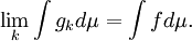
To illustrate some of the proof techniques used in Lebesgue integration theory, we sketch a proof of the above mentioned Lebesgue monotone convergence theorem:
Let {fk}k ∈ N be a non-decreasing sequence of non-negative measurable functions and put

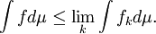
By the monotonicity property of the integral, it is immediate that:
and the limit on the right exists, since the sequence is monotonic.
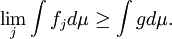
We now prove the inequality in the other direction (which also follows from Fatou's lemma), that is
It follows from the definition of integral, that there is a non-decreasing sequence gn of non-negative simple functions which converges to f pointwise almost everywhere and such that
Therefore, it suffices to prove that for each k ∈ N,
We will show that if g is a simple function and
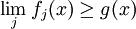
almost everywhere, then
By breaking up the function g into its constant value parts, this reduces to the case in which g is the indicator function of a set. The result we have to prove is then
- Suppose A is a measurable set and {fk}k ∈ N is a nondecreasing sequence of measurable functions on E such that
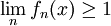
- for almost all x ∈ A. Then
To prove this result, fix ε > 0 and define the sequence of measurable sets

By monotonicity of the integral, it follows that for any n ∈ N,
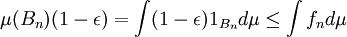
By assumption,

up to a set of measure 0. Thus by countable additivity of μ
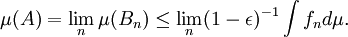
As this is true for any positive ε the result follows.
Alternative formulations
It is possible to develop the integral with respect to the Lebesgue measure without relying on the full machinery of measure theory. One such approach is provided by Daniell integral.
There is also an alternative approach to developing the theory of integration via methods of functional analysis. The Riemann integral exists for any continuous function f of compact support defined on Rn (or a fixed open subset). Integrals of more general functions can be built starting from these integrals. Let Cc be the space of all real-valued compactly supported continuous functions of R. Define a norm on Cc by
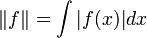
Then Cc is a normed vector space (and in particular, it is a metric space.) All metric spaces have Hausdorff completions, so let L1 be its completion. This space is isomorphic to the space of Lebesgue integrable functions modulo the subspace of functions with integral zero. Furthermore, the Riemann integral ∫ is uniformly continuous functional with respect to the norm on Cc, which is dense in L1. Hence ∫ has a unique extension to all of L1. This integral is precisely the Lebesgue integral.
This approach can be generalised to build the theory of integration with respect to Radon measures on locally compact spaces. It is the approach adopted by Bourbaki (2004); for more details see Radon measures on locally compact spaces.
Applications, e.g. in functional analysis
Finally one should of course mention that many statements on topological vector spaces (e.g. Hilbert or Banach spaces) and on limiting procedures therein (e.g. strong or weak convergence) are essentially simplified by using from the beginning the Lebesgue integral.