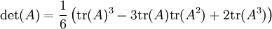
Determinant
2008/9 Schools Wikipedia Selection. Related subjects: Mathematics
In algebra, a determinant is a function depending on n that associates a scalar, det(A), to every n×n square matrix A. The fundamental geometric meaning of a determinant is as the scale factor for volume when A is regarded as a linear transformation. Determinants are important both in calculus, where they enter the substitution rule for several variables, and in multilinear algebra.
For a fixed positive integer n, there is a unique determinant function for the n×n matrices over any commutative ring R. In particular, this function exists when R is the field of real or complex numbers.
Vertical bar notation
The determinant of a matrix A is also sometimes denoted by |A|. This notation can be ambiguous since it is also used for certain matrix norms and for the absolute value. However, often the matrix norm will be denoted with double vertical bars (e.g., ‖A‖) and may carry a subscript as well. Thus, the vertical bar notation for determinant is frequently used (e.g., Cramer's rule and minors). For example, for matrix
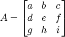
the determinant det(A) might be indicated by | A | or more explicitly as
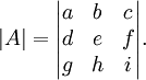
That is, the square braces around the matrices are replaced with elongated vertical bars.
Determinants of 2-by-2 matrices

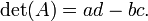
The 2×2 matrix

has determinant
The interpretation when the matrix has real number entries is that this gives the oriented area of the parallelogram with vertices at (0,0), (a,b), (a + c, b + d), and (c,d). The oriented area is the same as the usual area, except that it is negative when the vertices are listed in clockwise order.
The assumption here is that the linear transformation is applied to row vectors as the vector-matrix product xTA, where x is a column vector. The parallelogram in the figure is obtained by multiplying the row vectors  and
and  , defining the vertices of the unit square. With the more common matrix-vector product Ax the parallelogram has vertices at
 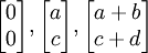 and
and  (note that Ax = (xTAT)T).
A formula for larger matrices will be given below.
Determinants of 3-by-3 matrices

The 3×3 matrix:
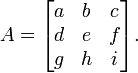
Using the cofactor expansion on the first row of the matrix we get:
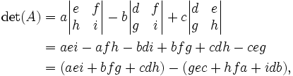

which can be remembered as the sum of the products of three diagonal north-west to south-east lines of matrix elements, minus the sum of the products of three diagonal south-west to north-east lines of elements when the copies of the first two columns of the matrix are written beside it as below:
Note that this mnemonic does not carry over into higher dimensions.
Applications
Determinants are used to characterize invertible matrices (i.e., exactly those matrices with non-zero determinants), and to explicitly describe the solution to a system of linear equations with Cramer's rule. They can be used to find the eigenvalues of the matrix A through the characteristic polynomial
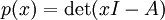
where I is the identity matrix of the same dimension as A.
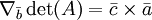
One often thinks of the determinant as assigning a number to every sequence of n vectors in  , by using the square matrix whose columns are the given vectors. With this understanding, the sign of the determinant of a basis can be used to define the notion of orientation in Euclidean spaces. The determinant of a set of vectors is positive if the vectors form a right-handed coordinate system, and negative if left-handed.
Determinants are used to calculate volumes in vector calculus: the absolute value of the determinant of real vectors is equal to the volume of the parallelepiped spanned by those vectors. As a consequence, if the linear map  is represented by the matrix A, and S is any measurable subset of , then the volume of f(S) is given by
 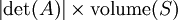 . More generally, if the linear map
  is represented by the m-by-n matrix A, and S is any measurable subset of
  , then the n- dimensional volume of f(S) is given by
  . By calculating the volume of the tetrahedron bounded by four points, they can be used to identify skew lines.
The volume of any tetrahedron, given its vertices a, b, c, and d, is (1/6)·|det(a − b, b − c, c − d)|, or any other combination of pairs of vertices that form a simply connected graph.
General definition and computation
The definition of the determinant comes from the following Theorem.
Theorem. Let Mn(K) denote the set of all  matrices over the field K. There exists exactly one function
with the two properties:
- F is alternating multilinear with regard to columns;
- F(I) = 1.
One can then define the determinant as the unique function with the above properties.
In proving the above theorem, one also obtains the Leibniz formula:
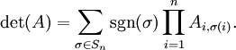
Here the sum is computed over all permutations σ of the numbers {1,2,...,n} and sgn(σ) denotes the signature of the permutation σ: +1 if σ is an even permutation and −1 if it is odd.
This formula contains n! (factorial) summands, and it is therefore impractical to use it to calculate determinants for large n.
For small matrices, one obtains the following formulas:
- if A is a 1-by-1 matrix, then
- if A is a 2-by-2 matrix, then

- for a 3-by-3 matrix A, the formula is more complicated:

which takes the shape of the Sarrus' scheme.
In general, determinants can be computed using Gaussian elimination using the following rules:
- If A is a triangular matrix, i.e.
 whenever i > j or, alternatively, whenever i < j, then
  (the product of the diagonal entries of A).
 - If B results from A by exchanging two rows or columns, then
- If B results from A by multiplying one row or column with the number c, then
- If B results from A by adding a multiple of one row to another row, or a multiple of one column to another column, then
Explicitly, starting out with some matrix, use the last three rules to convert it into a triangular matrix, then use the first rule to compute its determinant.
It is also possible to expand a determinant along a row or column using Laplace's formula, which is efficient for relatively small matrices. To do this along row i, say, we write
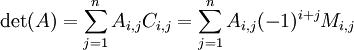
where the Ci,j represent the matrix cofactors, i.e. Ci,j is ( − 1)i + j times the minor Mi,j, which is the determinant of the matrix that results from A by removing the i-th row and the j-th column.
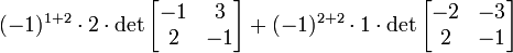
Example
Suppose we want to compute the determinant of
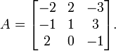
We can go ahead and use the Leibniz formula directly:


Alternatively, we can use Laplace's formula to expand the determinant along a row or column. It is best to choose a row or column with many zeros, so we will expand along the second column:

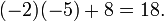
A third way (and the method of choice for larger matrices) would involve the Gauss algorithm. When doing computations by hand, one can often shorten things dramatically by cleverly adding multiples of columns or rows to other columns or rows; this does not change the value of the determinant, but may create zero entries which simplifies the subsequent calculations. In this example, adding the second column to the first one is especially useful:

and this determinant can be quickly expanded along the first column:

Properties
The determinant is a multiplicative map in the sense that
 for all n-by-n matrices A and B.
This is generalized by the Cauchy-Binet formula to products of non-square matrices.
It is easy to see that  and thus
 for all n-by-n matrices A and all scalars r.
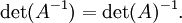
A matrix over a commutative ring R is invertible if and only if its determinant is a unit in R. In particular, if A is a matrix over a field such as the real or complex numbers, then A is invertible if and only if det(A) is not zero. In this case we have
Expressed differently: the vectors v1,...,vn in Rn form a basis if and only if det(v1,...,vn) is non-zero.
A matrix and its transpose have the same determinant:
The determinants of a complex matrix and of its conjugate transpose are conjugate:
(Note the conjugate transpose is identical to the transpose for a real matrix)
The determinant of a matrix A exhibits the following properties under elementary matrix transformations of A:
- Exchanging rows or columns multiplies the determinant by −1.
- Multiplying a row or column by m multiplies the determinant by m.
- Adding a multiple of a row or column to another leaves the determinant unchanged.
This follows from the multiplicative property and the determinants of the elementary matrix transformation matrices.
If A and B are similar, i.e., if there exists an invertible matrix X such that A = X − 1BX, then by the multiplicative property,
This means that the determinant is a similarity invariant. Because of this, the determinant of some linear transformation T : V → V for some finite dimensional vector space V is independent of the basis for V. The relationship is one-way, however: there exist matrices which have the same determinant but are not similar.
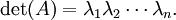
If A is a square n-by-n matrix with real or complex entries and if λ1,...,λn are the (complex) eigenvalues of A listed according to their algebraic multiplicities, then
This follows from the fact that A is always similar to its Jordan normal form, an upper triangular matrix with the eigenvalues on the main diagonal.
Useful identities
For m-by-n matrix A and m-by-n matrix B, it holds
- det(In + ATB) = det(Im + ABT) = det(In + BTA) = det(Im + BAT).
A consequence of these equalities for the case of (column) vectors x and y
- det(I + xyT) = 1 + yTx.
And a generalized version of this identity

Proofs can be found in .
Block matrices
Suppose, A,B,C,D are  matrices respectively. Then
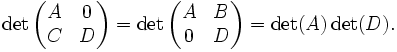
This can be (quite) easily seen from e.g. the Leibniz formula. Employing the following identity
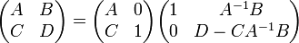
leads to
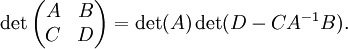
Similar identity with det(D) factored out can be derived analogously. These identities were taken from .
If dij are diagonal matrices, then
This is a special case of the theorem published in .
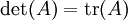
Relationship to trace
From this connection between the determinant and the eigenvalues, one can derive a connection between the trace function, the exponential function, and the determinant:

Performing the substitution  in the above equation yields

which is closely related to the Fredholm determinant. Similarly,

For n-by-n matrices there are the relationships:
- Case n = 1:
- Case n = 2:
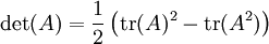
- Case n = 3:
- Case n = 4:


which are closely related to Newton's identities.
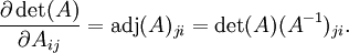
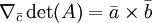
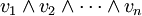
Derivative
The determinant of real square matrices is a polynomial function from  to
to  , and as such is everywhere differentiable. Its derivative can be expressed using Jacobi's formula:

where adj(A) denotes the adjugate of A. In particular, if A is invertible, we have

In component form, these are
When ε is a small number these are equivalent to

The special case where A is equal to the identity matrix I yields

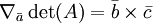
A useful property in the case of 3 x 3 matrices is the following:
A may be written as  where
where  ,
,  ,
,  are vectors, then the gradient over one of the three vectors may be written as the cross product of the other two:
Abstract formulation
An n × n square matrix A may be thought of as the coordinate representation of a linear transformation of an n-dimensional vector space V. Given any linear transformation

we can define the determinant of A as the determinant of any matrix representation of A. This is a well-defined notion (i.e. independent of a choice of basis) since the determinant is invariant under similarity transformations.
As one might expect, it is possible to define the determinant of a linear transformation in a coordinate-free manner. If V is an n-dimensional vector space, then one can construct its top exterior power ΛnV. This is a one-dimensional vector space whose elements are written
where each vi is a vector in V and the wedge product ∧ is antisymmetric (i.e., u∧u = 0). Any linear transformation A : V → V induces a linear transformation of ΛnV as follows:

Since ΛnV is one-dimensional this operation is just multiplication by some scalar that depends on A. This scalar is called the determinant of A. That is, we define det(A) by the equation

One can check that this definition agrees with the coordinate-dependent definition given above.
Algorithmic implementation
- The naive method of implementing an algorithm to compute the determinant is to use Laplace's formula for expansion by cofactors. This approach is extremely inefficient in general, however, as it is of order n! (n factorial) for an n×n matrix M.
- An improvement to order n3 can be achieved by using LU decomposition to write M = LU for triangular matrices L and U. Now, det M = det LU = det L det U, and since L and U are triangular the determinant of each is simply the product of its diagonal elements. Alternatively one can perform the Cholesky decomposition if possible or the QR decomposition and find the determinant in a similar fashion.
- Since the definition of the determinant does not need divisions, a question arises: do fast algorithms exist that do not need divisions? This is especially interesting for matrices over rings. Indeed algorithms with run-time proportional to n4 exist. An algorithm of Mahajan and Vinay, and Berkowitz is based on closed ordered walks (short clow). It computes more products than the determinant definition requires, but some of these products cancel and the sum of these products can be computed more efficiently. The final algorithm looks very much like an iterated product of triangular matrices.
- What is not often discussed is the so-called "bit complexity" of the problem, i.e. how many bits of accuracy you need to store for intermediate values. For example, using Gaussian elimination, you can reduce the matrix to upper triangular form, then multiply the main diagonal to get the determinant (this is essentially a special case of the LU decomposition as above), but a quick calculation will show that the bit size of intermediate values could potentially become exponential. One could talk about when it is appropriate to round intermediate values, but an elegant way of calculating the determinant uses the Bareiss Algorithm, an exact-division method based on Sylvester's identity to give a run time of order n3 and bit complexity roughly the bit size of the original entries in the matrix times n.
History
Historically, determinants were considered before matrices. Originally, a determinant was defined as a property of a system of linear equations. The determinant "determines" whether the system has a unique solution (which occurs precisely if the determinant is non-zero). In this sense, determinants were first used in the 3rd century BC Chinese math textbook The Nine Chapters on the Mathematical Art. In Europe, two-by-two determinants were considered by Cardano at the end of the 16th century and larger ones by Leibniz and, in Japan, by Seki about 100 years later. Cramer (1750) added to the theory, treating the subject in relation to sets of equations. The recurrent law was first announced by Bézout (1764).
It was Vandermonde (1771) who first recognized determinants as independent functions. Laplace (1772) gave the general method of expanding a determinant in terms of its complementary minors: Vandermonde had already given a special case. Immediately following, Lagrange (1773) treated determinants of the second and third order. Lagrange was the first to apply determinants to questions elimination theory; he proved many special cases of general identities.
Gauss (1801) made the next advance. Like Lagrange, he made much use of determinants in the theory of numbers. He introduced the word determinants (Laplace had used resultant), though not in the present signification, but rather as applied to the discriminant of a quantic. Gauss also arrived at the notion of reciprocal (inverse) determinants, and came very near the multiplication theorem.
The next contributor of importance is Binet (1811, 1812), who formally stated the theorem relating to the product of two matrices of m columns and n rows, which for the special case of m = n reduces to the multiplication theorem. On the same day ( November 30, 1812) that Binet presented his paper to the Academy, Cauchy also presented one on the subject. (See Cauchy-Binet formula.) In this he used the word determinant in its present sense, summarized and simplified what was then known on the subject, improved the notation, and gave the multiplication theorem with a proof more satisfactory than Binet's. With him begins the theory in its generality.
The next important figure was Jacobi (from 1827). He early used the functional determinant which Sylvester later called the Jacobian, and in his memoirs in Crelle for 1841 he specially treats this subject, as well as the class of alternating functions which Sylvester has called alternants. About the time of Jacobi's last memoirs, Sylvester (1839) and Cayley began their work.
The study of special forms of determinants has been the natural result of the completion of the general theory. Axisymmetric determinants have been studied by Lebesgue, Hesse, and Sylvester; persymmetric determinants by Sylvester and Hankel; circulants by Catalan, Spottiswoode, Glaisher, and Scott; skew determinants and Pfaffians, in connection with the theory of orthogonal transformation, by Cayley; continuants by Sylvester; Wronskians (so called by Muir) by Christoffel and Frobenius; compound determinants by Sylvester, Reiss, and Picquet; Jacobians and Hessians by Sylvester; and symmetric gauche determinants by Trudi. Of the text-books on the subject Spottiswoode's was the first. In America, Hanus (1886), Weld (1893), and Muir/Metzler (1933) published treatises.